44 show data labels excel
How to use data labels in a chart - YouTube Excel charts have a flexible system to display values called "data labels". Data labels are a classic example a "simple" Excel feature with a huge range of o... › xlpivot05Fix Excel Pivot Table Missing Data Field Settings Aug 31, 2022 · Show Missing Data. To show missing data, such as new products, you can add one or more dummy records to the pivot table, to force the items to appear. For example, to include a new product -- Paper -- in the pivot table, even if it has not yet been sold: In the source data, add a record with Paper as the product, and 0 as the quantity; Refresh ...
Add data labels and callouts to charts in Excel 365 - EasyTweaks.com Step #1: After generating the chart in Excel, right-click anywhere within the chart and select Add labels . Note that you can also select the very handy option of Adding data Callouts. Step #2: When you select the "Add Labels" option, all the different portions of the chart will automatically take on the corresponding values in the table ...

Show data labels excel
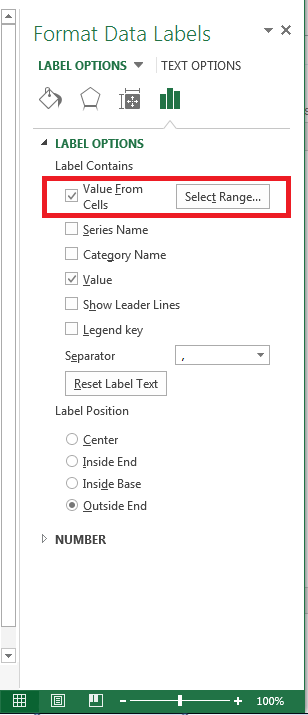
How to add data labels from different column in an Excel chart? Right click the data series, and select Format Data Labels from the context menu. 3. In the Format Data Labels pane, under Label Options tab, check the Value From Cells option, select the specified column in the popping out dialog, and click the OK button. Now the cell values are added before original data labels in bulk. 4. How to Add Data Labels in Excel - Excelchat | Excelchat In Excel 2013 and the later versions we need to do the followings; Click anywhere in the chart area to display the Chart Elements button Figure 5. Chart Elements Button Click the Chart Elements button > Select the Data Labels, then click the Arrow to choose the data labels position. Figure 6. How to Add Data Labels in Excel 2013 Figure 7. How to I rotate data labels on a column chart so that they are ... Thanks for your query in this community. To change the text direction, first of all, please double click on the data label and make sure the data are selected (with a box surrounded like following image). Then on your right panel, the Format Data Labels panel should be opened. Go to Text Options > Text Box > Text direction > Rotate
Show data labels excel. Excel, giving data labels to only the top/bottom X% values 1) Create a data set next to your original series column with only the values you want labels for (again, this can be formula driven to only select the top / bottom n values). See column D below. 2) Add this data series to the chart and show the data labels. 3) Set the line color to No Line, so that it does not appear! 4) Volia! See Below! Share How to add data labels in excel to graph or chart (Step-by-Step) Add data labels to a chart. 1. Select a data series or a graph. After picking the series, click the data point you want to label. 2. Click Add Chart Element Chart Elements button > Data Labels in the upper right corner, close to the chart. 3. Click the arrow and select an option to modify the location. 4. Excel tutorial: How to use data labels Generally, the easiest way to show data labels to use the chart elements menu. When you check the box, you'll see data labels appear in the chart. If you have more than one data series, you can select a series first, then turn on data labels for that series only. You can even select a single bar, and show just one data label. Adding Data Labels to Your Chart (Microsoft Excel) - ExcelTips (ribbon) Make sure the Layout tab of the ribbon is displayed. Click the Data Labels tool. Excel displays a number of options that control where your data labels are positioned. Select the position that best fits where you want your labels to appear. To add data labels in Excel 2013 or later versions, follow these steps:
how to add data labels into Excel graphs - storytelling with data You can download the corresponding Excel file to follow along with these steps: Right-click on a point and choose Add Data Label. You can choose any point to add a label—I'm strategically choosing the endpoint because that's where a label would best align with my design. Excel defaults to labeling the numeric value, as shown below. Custom Chart Data Labels In Excel With Formulas - How To Excel At Excel Follow the steps below to create the custom data labels. Select the chart label you want to change. In the formula-bar hit = (equals), select the cell reference containing your chart label's data. In this case, the first label is in cell E2. Finally, repeat for all your chart laebls. Excel charts: how to move data labels to legend @Matt_Fischer-Daly . You can't do that, but you can show a data table below the chart instead of data labels: Click anywhere on the chart. On the Design tab of the ribbon (under Chart Tools), in the Chart Layouts group, click Add Chart Element > Data Table > With Legend Keys (or No Legend Keys if you prefer) Add or remove data labels in a chart - Microsoft Support Right-click the data series or data label to display more data for, and then click Format Data Labels. Click Label Options and under Label Contains, select the Values From Cells checkbox. When the Data Label Range dialog box appears, go back to the spreadsheet and select the range for which you want the cell values to display as data labels.
chandoo.org › wp › change-data-labels-in-chartsHow to Change Excel Chart Data Labels to Custom Values? May 05, 2010 · Now, click on any data label. This will select “all” data labels. Now click once again. At this point excel will select only one data label. Go to Formula bar, press = and point to the cell where the data label for that chart data point is defined. Repeat the process for all other data labels, one after another. See the screencast. Find, label and highlight a certain data point in Excel scatter graph Select the Data Labels box and choose where to position the label. By default, Excel shows one numeric value for the label, y value in our case. To display both x and y values, right-click the label, click Format Data Labels…, select the X Value and Y value boxes, and set the Separator of your choosing: Label the data point by name Displaying Large Numbers in K (thousands) or M (millions) in Excel How To Display Numbers in Millions in Excel Right-Click any number you want to convert. Go to Format Cells. In the pop-up window, move to Custom formatting. If you want to show the numbers in Millions, simply change the format from General to 0,,"M" . The figures will now be 23M. Change the format of data labels in a chart To get there, after adding your data labels, select the data label to format, and then click Chart Elements > Data Labels > More Options. To go to the appropriate area, click one of the four icons ( Fill & Line, Effects, Size & Properties ( Layout & Properties in Outlook or Word), or Label Options) shown here.
Total of chart series – Excel kitchenette
How to create Custom Data Labels in Excel Charts - Efficiency 365 Create the chart as usual. Add default data labels. Click on each unwanted label (using slow double click) and delete it. Select each item where you want the custom label one at a time. Press F2 to move focus to the Formula editing box. Type the equal to sign. Now click on the cell which contains the appropriate label.

axis vs data labels — storytelling with data
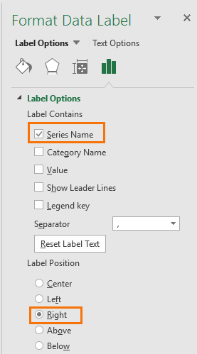
How to Customize Your Excel Pivot Chart Data Labels - dummies The Data Labels command on the Design tab's Add Chart Element menu in Excel allows you to label data markers with values from your pivot table. When you click the command button, Excel displays a menu with commands corresponding to locations for the data labels: None, Center, Left, Right, Above, and Below. None signifies that no data labels ...

Apply Custom Data Labels to Charted Points - Peltier Tech
› excel › how-to-add-total-dataHow to Add Total Data Labels to the Excel Stacked Bar Chart Apr 03, 2013 · Step 4: Right click your new line chart and select “Add Data Labels” Step 5: Right click your new data labels and format them so that their label position is “Above”; also make the labels bold and increase the font size. Step 6: Right click the line, select “Format Data Series”; in the Line Color menu, select “No line”

Improve your X Y Scatter Chart with custom data labels
Show Data Label in Excel Chart Only When Data Point is selected/hovered ... Show Data Label in Excel Chart Only When Data Point is selected/hovered over Hi there, Does anyone know if it is possible to set Data Labels that are pointing to a range of selected cells and not just coming natively from the data point, in an Excel Chart so that they only appear if the user clicks on the data point or maybe hovers on it? ...

Add data labels and callouts to charts in Excel 365 ...
_Chart.ShowDataLabelsOverMaximum Property (Microsoft.Office.Interop.Excel) In this article. Definition. Remarks. Applies to. Returns or sets whether to show the data labels when the value is greater than the maximum value on the value axis. Read/write. C#. Copy.
Dynamically Label Excel Chart Series Lines • My Online ...
How to Add Data Labels to an Excel 2010 Chart - dummies On the Chart Tools Layout tab, click Data Labels→More Data Label Options. The Format Data Labels dialog box appears. You can use the options on the Label Options, Number, Fill, Border Color, Border Styles, Shadow, Glow and Soft Edges, 3-D Format, and Alignment tabs to customize the appearance and position of the data labels.
How to show the percentage on stacked colum/bar chart in ...
How to show data label in "percentage" instead of - Microsoft Community Select Format Data Labels Select Number in the left column Select Percentage in the popup options In the Format code field set the number of decimal places required and click Add. (Or if the table data in in percentage format then you can select Link to source.) Click OK Regards, OssieMac Report abuse 8 people found this reply helpful ·

Custom data labels in a chart
› how-to-create-excel-pie-chartsHow to Make a Pie Chart in Excel & Add Rich Data Labels to ... Sep 08, 2022 · Excel Pie Chart Labels on Slices: Add, Show & Modify Factors; How to Change Pie Chart Colors in Excel (4 Easy Ways) Add Labels with Lines in an Excel Pie Chart (with Easy Steps) How to Edit Pie Chart in Excel (All Possible Modifications) Create A Doughnut, Bubble and Pie of Pie Chart in Excel; How to Make a Pie Chart with Multiple Data in Excel ...

Microsoft Excel Tutorials: Add Data Labels to a Pie Chart
› 509290 › how-to-use-cell-valuesHow to Use Cell Values for Excel Chart Labels - How-To Geek Mar 12, 2020 · Make your chart labels in Microsoft Excel dynamic by linking them to cell values. When the data changes, the chart labels automatically update. In this article, we explore how to make both your chart title and the chart data labels dynamic. We have the sample data below with product sales and the difference in last month’s sales.
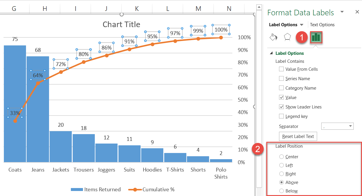
How to Create a Pareto Chart in Excel – Automate Excel
› how-to-show-percentage-inHow to Show Percentage in Pie Chart in Excel? - GeeksforGeeks Jun 29, 2021 · It can be observed that the pie chart contains the value in the labels but our aim is to show the data labels in terms of percentage. Show percentage in a pie chart: The steps are as follows : Select the pie chart. Right-click on it. A pop-down menu will appear. Click on the Format Data Labels option. The Format Data Labels dialog box will appear.
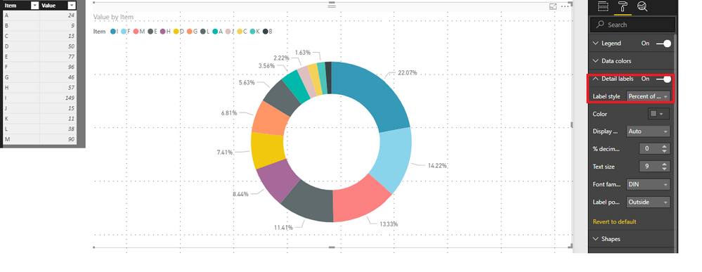
Solved: How to show all detailed data labels of pie chart ...
How to hide zero data labels in chart in Excel? - ExtendOffice If you want to hide zero data labels in chart, please do as follow: 1. Right click at one of the data labels, and select Format Data Labels from the context menu. See screenshot: 2. In the Format Data Labels dialog, Click Number in left pane, then select Custom from the Category list box, and type #"" into the Format Code text box, and click Add button to add it to Type list box.

How to Use Cell Values for Excel Chart Labels
to display top 5 data labels on graph [SOLVED] Re: to display top 5 data labels on graph. Also, I noticed your sum column ("total") is returning errors. I don't see why you would want to do this, and in fact I'm not even sure why excel wanted to do this to begin with. if you run C3+D3 when those cells are empty, excel should return 0. So I got rid of the error, and that way, you can use the ...

Add or remove data labels in a chart
Add a DATA LABEL to ONE POINT on a chart in Excel Steps shown in the video above: Click on the chart line to add the data point to. All the data points will be highlighted. Click again on the single point that you want to add a data label to. Right-click and select ' Add data label ' This is the key step! Right-click again on the data point itself (not the label) and select ' Format data label '.
What's the difference between 'show labels' and 'show values ...
How To Add Data Labels In Excel - veganheath.info To get there, after adding your data labels, select the data label to format, and then click chart elements > data labels > more options. After picking the series, click the data point you want to label. Source: temotips.blogspot.com. Using excel chart element button to add axis labels. Click the chart to show the chart elements button.

Excel Charts - Aesthetic Data Labels
Format Data Labels in Excel- Instructions - TeachUcomp, Inc. To do this, click the "Format" tab within the "Chart Tools" contextual tab in the Ribbon. Then select the data labels to format from the "Chart Elements" drop-down in the "Current Selection" button group. Then click the "Format Selection" button that appears below the drop-down menu in the same area.

Add or remove data labels in a chart
› 682077 › how-to-rename-a-dataHow to Rename a Data Series in Microsoft Excel - How-To Geek Jul 27, 2020 · A data series in Microsoft Excel is a set of data, shown in a row or a column, which is presented using a graph or chart. To help analyze your data, you might prefer to rename your data series. Rather than renaming the individual column or row labels, you can rename a data series in Excel by editing the graph or chart.
Showing Cell Range as the Data Labels|Documentation
How to I rotate data labels on a column chart so that they are ... Thanks for your query in this community. To change the text direction, first of all, please double click on the data label and make sure the data are selected (with a box surrounded like following image). Then on your right panel, the Format Data Labels panel should be opened. Go to Text Options > Text Box > Text direction > Rotate

Adding rich data labels to charts in Excel 2013 | Microsoft ...
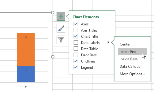
How to Add Data Labels in Excel - Excelchat | Excelchat In Excel 2013 and the later versions we need to do the followings; Click anywhere in the chart area to display the Chart Elements button Figure 5. Chart Elements Button Click the Chart Elements button > Select the Data Labels, then click the Arrow to choose the data labels position. Figure 6. How to Add Data Labels in Excel 2013 Figure 7.

How to show percentages on three different charts in Excel ...
How to add data labels from different column in an Excel chart? Right click the data series, and select Format Data Labels from the context menu. 3. In the Format Data Labels pane, under Label Options tab, check the Value From Cells option, select the specified column in the popping out dialog, and click the OK button. Now the cell values are added before original data labels in bulk. 4.

Add or remove data labels in a chart

How to Show Percentage in Pie Chart in Excel? - GeeksforGeeks
Format Data Label: Label Position - Microsoft Community

Excel charts: add title, customize chart axis, legend and ...

How to Change Excel Chart Data Labels to Custom Values?

How to Use Cell Values for Excel Chart Labels

Solved: How to show all detailed data labels of pie chart ...

Excel Charts: Dynamic Label positioning of line series

Add or remove data labels in a chart
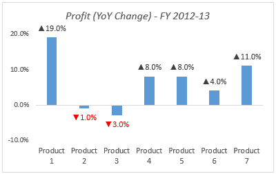
Color Negative Chart Data Labels in Red with downward arrow

How to Place Labels Directly Through Your Line Graph in ...

Format Number Options for Chart Data Labels in PowerPoint ...

microsoft excel - Adding data label only to the last value ...
/Capture-e92aa05671d543ceaf94080eb2687619.JPG)
Understanding Excel Chart Data Series, Data Points, and Data ...

Change the format of data labels in a chart

How to Make Pie Chart with Labels both Inside and Outside ...

Chart axes, legend, data labels, trendline in Excel - Tech Funda

microsoft excel - Adding data label only to the last value ...

How to add or move data labels in Excel chart?

How to add or move data labels in Excel chart?

Adding rich data labels to charts in Excel 2013 | Microsoft ...
/simplexct/BlogPic-f7888.png)
How to Add Labels to Show Totals in Stacked Column Charts in ...

Google Workspace Updates: Get more control over chart data ...

How to add data labels from different column in an Excel chart?

How to add live total labels to graphs and charts in Excel ...
Post a Comment for "44 show data labels excel"